A common problem solving strategy consists in decomposing a problem into subproblems, so that either all or just one of these subproblems need to be solved in order to obtain a solution for the original problem. Representing each problem as a node in a directed graph, where arcs express the decomposition relationship between problems and subproblems, two kinds of nodes arise related to both types of decomposition, AND nodes and OR nodes, and the obtained structure is an AND/OR graph. Certain subproblems, depicted in the graph as terminal nodes, can be solved directly, and a solution for the original problem (corresponding to the root node in the graph) can be found by applying graph searching techniques. The solution consists of a subgraph that relates the root node to one or several terminal nodes. Terminal nodes are leaf nodes, i.e., nodes without successors. Another kind of leaf nodes are the non-terminal leaf nodes which represent elementary subproblems that have no solution. Obviously such nodes cannot appear in a solution subgraph.
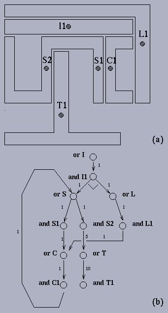
The cyclic nature of many AND/OR graphs corresponding to different problem types becomes evident in the following example, which can be viewed as a special kind of disassembly problem (AND/OR graphs are frequently used representations in the assembly/disassembly and grasping contexts). A given workpiece laying among other different workpieces has to be picked up, and this can only be done if at least one of the gripping points of that workpiece is free, i.e. no other workpieces obstructing the access to such point (Figure (a)). Obstructing workpieces have to be removed, but their gripping points may in turn be obstructed by other workpieces. For example, point I1 of piece "I" is obstructed by pieces "L" and "S", thus these pieces have to be taken away first, but their gripping points are also obstructed by other pieces. This problem has clearly an AND/OR structure: every workpiece corresponds to an OR node, for it can be picked up by either of its gripping points (the successors of this OR node), which are represented by AND nodes, as far as all workpieces obstructing this point have to be taken away (Figure (b)). The costs of the arcs have been set arbitrarily in this example, but they could reflect physical facts. Now, consider the situation where an obstructing workpiece in its turn is obstructed by the obstructed workpiece or one of its ancestors. This clearly corresponds to a cycle in the graph. Observe that points S1 and C1 are obstructing each other, and, indeed, a cycle exists that contains the corresponding nodes.

These books appear in (almost) every bibliography:

A straightforward but highly inefficient way to solve cyclic AND/OR graphs consists in "unfolding" the cycles, while applying an algorithm for acyclic graphs. This can lead to a large waste of computer effort if the arcs of the cycle have comparatively small cost with respect to the solution (if one exists), or to an infinite loop, if there are no alternatives to the cycles. Nonetheless, before tackling cyclic AND/OR graphs, it is advisable to learn something about the easier problem of solving acyclic graphs. These references describe some efficient algorithms for solving implicit AND/OR graphs. In particular, Mahanti and Bagchi's CF algorithm has inspired the top-down search strategy of our CFCREV* algorithm for cyclic graphs, as well as the use of arc markings for restricting the cost revision process to a subset of the whole explicit graph.
Solving cyclic graphs is a qualitatively much harder problem. Hvalica's work constitute a very clear and formal approach to the behaviour of the "classical" AO* algorithm in cyclic graphs, its key contribution being a neat modification of the cost revision process that permits handling cycles. Efficiency, however, is not an issue addressed in this work and, thus, the revision process --which extends to all ancestors of the expanded node-- turns out to be more expensive than necessary. Kumar's algorithm works bottom-up on explicit graphs with cycles. It is very efficient, but bottom-up strategies have a drawback that can be important in particular settings: the need of generating all terminal nodes, although most of them will not intervene in the solution. Moreover, they cannot be applied if the search for a solution and the graph construction are simultaneously performed. Up to date, the best performance is obtained with Chakrabarti's algorithms, which have been originally developed for explicit graphs, but can be adapted to work on implicit graphs, as suggested by the author. However, some drawbacks appear to be attached these procedures when applied to implicit graphs, which are overcome in our CFCREV*. The cost revision strategy of our algorithm is based on Chakrabarti's REV*.

Consider the explicit graph at a given instant (initially it will consist only of the start node. At each iteration of the search process, the explicit graph is expanded in a top-down fashion. Like AO*, this algorithm has the property that at every moment, below each node "n" exactly one of the potential solution graphs (psg) is marked; we call this the marked psg below "n". Exactly one of the outgoing arcs of every OR node that belongs to this psg is marked, whereas, in the case of AND nodes, all arcs pointing to their successors are marked. By the marked psg we mean the marked psg below the start node. Cost estimates "F" are revised bottom-up, but only along marked arcs. During the cost revision process, arc-marking changes may occur at OR nodes along the currently marked psg, leading to an alternative, more promising, marked psg. The search for the minimum-cost solution graph is performed in four main steps, which are repeated until the solution is found or it is determined that no solution exists:
More details about the algorithm, a pseudocode description, as well as formal proofs of its validity and efficiency will soon be available.
If you want to test the algorithm, just press the SHIFT key and click here for downloading the executable (the source has been written in ANSI C).
CFC is an efficient algorithm that solves graphs containing cycles. In order to test how it works, an implicit graph has to be provided. The algorithm then determines at each execution of its main loop the explicit graph expanded so far, as well as the current solution. Each one of these executions correspond to the expansion of a tip node, and the algorithm finishes as soon as all the tip nodes of the solution subgraph (all the arcs that belong to the current solution subgraph are "marked") are solved terminal nodes. If no solution actually exists, e.g. if all possible alternatives lead to unsolvable cycles, then the algorithm finishes reporting that the root node is unsolved and its cost estimate is equal to infinite.
The algorithm has been compiled on a Sun Solaris and can be executed with the command
cfc Templates for the input file are provided with the examples.
The nodes of the graph have to contain some information, concerning
their AND/OR nature, whether they are terminal nodes or not, and the
value of their heuristic estimators. As for the topology of the graph,
the cost and directions of each arc, toghether with the nodes it
connects, must also be known. We have decided to provide all these
data in a straightforward, obviously improvable way. The example given
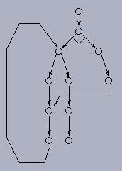
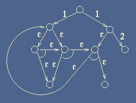
below corresponds to the input file "example", and the graph is also
depicted. Adjacency and incidency matrices are the most common ways of
describing the topological relationships graphs. It should not be very
difficult to derive an interface for translating these formats into the
naďf form of the corresponding part in our input files. The input format is self-explanatory (it corresponds to the graph in
the figure above):
Number_of_nodes 11
visiting AND vertex 0 Last Modified on friday, May 12, 1998
This command can be executed with the -i option, which allows to follow the evolution
of the marked psg along the iterations of the main loop.
Input format
h(0) 1
AND(0)/OR(1) 1
SOLVED(0)/NON_TERMINAL(1) 1
h(1) 1
AND(0)/OR(1) 0
SOLVED(0)/NON_TERMINAL(1) 1
h(2) 1
AND(0)/OR(1) 1
SOLVED(0)/NON_TERMINAL(1) 1
h(3) 0
AND(0)/OR(1) 1
SOLVED(0)/NON_TERMINAL(1) 1
h(4) 1
AND(0)/OR(1) 0
SOLVED(0)/NON_TERMINAL(1) 1
h(5) 1
AND(0)/OR(1) 0
SOLVED(0)/NON_TERMINAL(1) 1
h(6) 0
AND(0)/OR(1) 0
SOLVED(0)/NON_TERMINAL(1) 1
h(7) 2
AND(0)/OR(1) 1
SOLVED(0)/NON_TERMINAL(1) 1
h(8) 0
AND(0)/OR(1) 1
SOLVED(0)/NON_TERMINAL(1) 1
h(9) 1
AND(0)/OR(1) 0
SOLVED(0)/NON_TERMINAL(1) 1
h(10) 0
AND(0)/OR(1) 0
SOLVED(0)/NON_TERMINAL(1) 0
arcsarcsarcsarcsarcsarcsarcsarcsarcsarcsarcsarcs
vtx1 0
vtx2 1
weigth 1
another? 1
vtx1 1
vtx2 2
weigth 1
another? 1
vtx1 1
vtx2 3
weigth 1
another? 1
vtx1 2
vtx2 4
weigth 1
another? 1
vtx1 2
vtx2 5
weigth 1
another? 1
vtx1 3
vtx2 6
weigth 1
another? 1
vtx1 4
vtx2 7
weigth 1
another? 1
vtx1 5
vtx2 8
weigth 5
another? 1
vtx1 6
vtx2 7
weigth 1
another? 1
vtx1 7
vtx2 9
weigth 1
another? 1
vtx1 8
vtx2 10
weigth 10
another? 1
vtx1 9
vtx2 2
weigth 1
another? 0
First the total number of nodes is introduced. For each node "n", the
value of the heuristic estimator h(n) is given, as well as its AND/OR
and SOLVED/NON_TERMINAL nature (non-solvable leaf nodes are not
considered). Then the data concerning the arcs are entered: the parent
and the child node connected by the arc (vtx1 and vtx2 respectively,
thus the direction is implicitly provided), as well as the weight or
cost of the arc. Finally, it is asked whether another arc has to be
entered (1) or not (0). In the latter case, the input finishes.
Output
The output of the algorithm consists in a description of the solution
graph as a sequence of nodes (following a depth-first order in the
graph) and, for each node, the following information is given:
whose status is SOLVED
costs are H 1.000000 and F 3.000000
which has following outgoing arcs:
a marked arc whose cost is 1.000000
connected to successor 1
a marked arc whose cost is 1.000000
connected to successor 2
visiting OR vertex 1
whose status is SOLVED
costs are H 0.000000 and F 2.000000
which has following outgoing arcs:
a marked arc whose cost is 1.000000
connected to successor 2
etc.
i.e., the type and identification number of the node, its
SOLVED/UNSOLVED/UNEXPANDED status, the values of its heuristic estimator and of its
cost estimator F, and a list of marked arcs pointing to its successors
(with their weights). The final status of the root node, the cost of the solution and
the total number of iterations of the main loop are also given.
If the algorithm is executed with the -i option, then the same information is given
for the nodes in the marked psg at each iteration. Furthermore, previously to the
description of each psg, the identification number is given of the node which is
going to be expanded.
Examples